3.3x Faster HuggingFace Tokenizers for Single Sequence
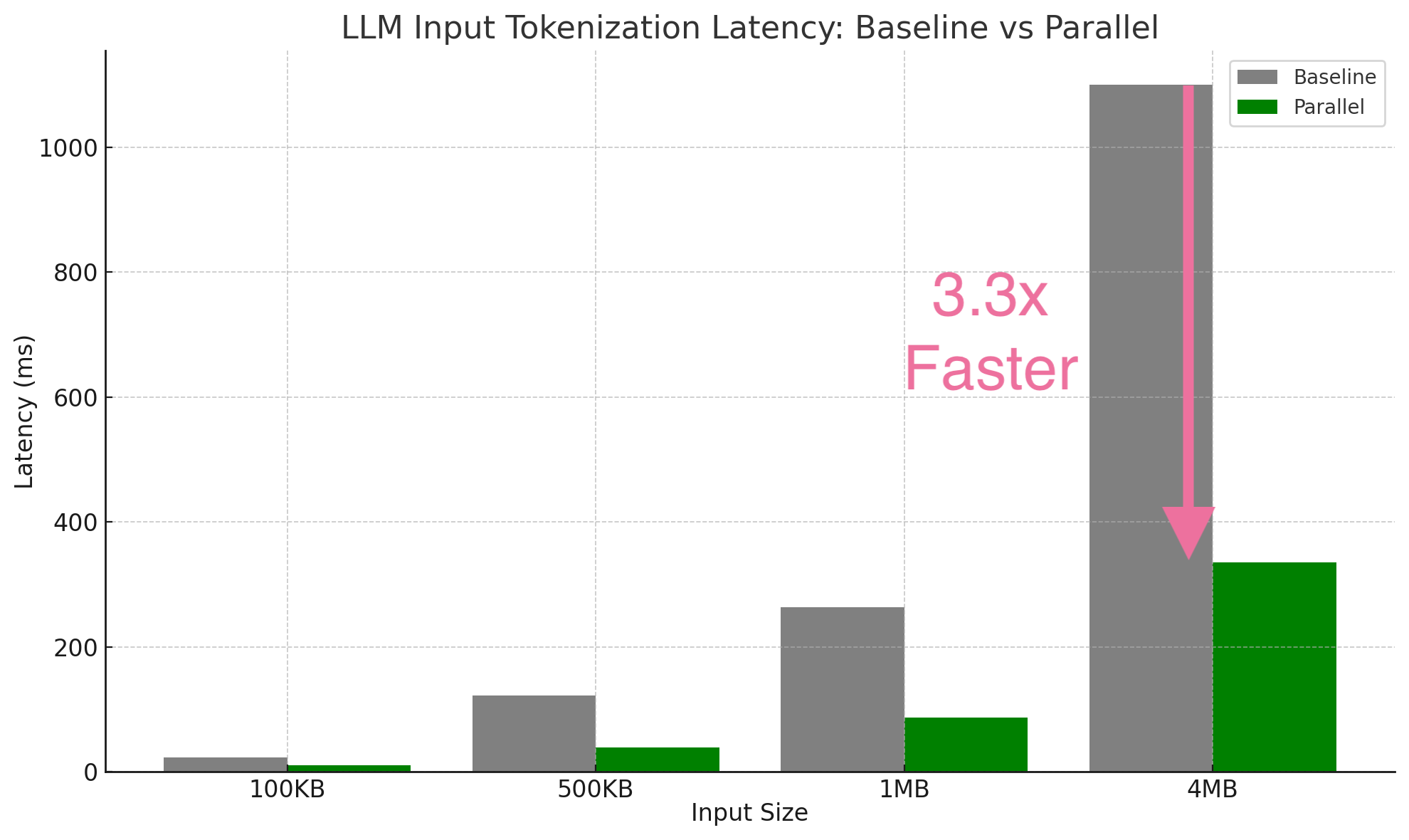
Table of Contents
I made HuggingFace tokenizers 3.3x faster by parallelizing single-input tokenization with overlapping chunks, zero-copy offset operations, SIMD-accelerated boundary detection, and cache-hierarchy-aware chunking. The result is bit-identical to serial encoding. Fast tokenization is critical to achieve low TTFT given long context.
The Long Context Revolution Has a Bottleneck
LLM models now routinely handle 1M+ token contexts. This isn’t just a bigger number; it’s enabling fundamentally new use cases:
- AI Agents: Load entire codebases into context instead of fumbling with RAG retrieval. Why search when you can reason over everything?
- Document Analysis: Process entire legal contracts, medical records, or research papers in one shot—no chunking, no context loss.
- Displacing RAG: Google’s “infinite context” approach suggests a future where retrieval augmentation becomes unnecessary.
But there’s a bottleneck nobody talks about: tokenization.
Everyone optimizes inference—quantization, KV cache, flash attention, speculative decoding, etc. But it takes 1.1 seconds to tokenize a 4MB document (about 1M tokens).
As AI agents scale with tool use and long context with multi-turns, the tokenization latency hurts TTFT (Time to First Token) and time to completion.
The challenge: Tokenization is inherently sequential. You process one token, then find the next, then the next. How to parallelize this without breaking correctness?
The Core Insight: Overlapping Chunks
The breakthrough is simple: we can chunk, parallelize, and merge.
The naive approach of splitting text and tokenizing in parallel doesn’t work, because you’ll get different results than serial encoding given tokens can span split boundaries. My solution uses overlapping chunks with a deterministic merge algorithm detailed in Appendix A.
Key Optimizations
Optimization 1: Recursive Divide-and-Conquer Strategy
We use binary splitting with rayon::join for work-stealing parallelism:
1
2
3
4
5
6
7
8
9
10
11
12
13
14
15
16
fn encode_recursive(input: &str, depth: usize, max_depth: usize) -> Encoding {
    if depth >= max_depth {
        return encode_serial(input);  // Base case
    }

    let mid = find_split_point(input, input.len() / 2);
    let (left_chunk, right_chunk) = create_overlapping_chunks(input, mid);

    // Parallel execution via rayon
    let (left_encoding, right_encoding) = rayon::join(
        || encode_recursive(left_chunk, depth + 1, max_depth),
        || encode_recursive(right_chunk, depth + 1, max_depth),
    );

    merge_at_midpoint(left_encoding, right_encoding, mid)
}
Auto-tuning depth based on input size and CPU cores:
- 100KB input → depth 2 (4 parallel chunks)
- 500KB input → depth 3 (8 parallel chunks)
- 1MB input → depth 4 (16 parallel chunks)
Why binary splitting? Clean merge semantics and work-stealing efficiency. Rayon automatically balances work across available cores.
Results: 1.7-2.1x speedup for 100KB-500KB inputs.
Sweet spot: Medium-sized documents like research papers, API documentation, or individual source files.
Optimization 2: Cache-Block Streaming for Large Inputs
At 1MB+, recursive splitting starts causing cache thrashing. Different threads access scattered memory regions, evicting each other’s data from cache.
The solution: Process input in L1-cache-sized blocks sequentially:
1
2
3
4
5
6
7
Input (1MB):
├───┬───┬───┬───┬───┬───┬───┬───┬───┬───┬───┬───┬───┬──────┤
│ 0 │ 1 │ 2 │ 3 │ 4 │ 5 │ 6 │ 7 │ 8 │ 9 │10 │11 │12 │ ...  │
│8KB│8KB│8KB│8KB│8KB│8KB│8KB│8KB│8KB│8KB│8KB│8KB│8KB│      │
└───┴───┴───┴───┴───┴───┴───┴───┴───┴───┴───┴───┴───┴──────┘
  ↓   ↓   ↓   ↓   ↓   ↓   ↓   ↓   ↓   ↓   ↓   ↓   ↓
  Encode all blocks in parallel, merge sequentially
Why 8KB blocks? We benchmarked extensively:
| Block Size | Time (4MB) | Throughput | vs 64KB |
|---|---|---|---|
| 4KB | 386ms | 10.4 MiB/s | +31% faster ⭐ |
| 8KB | 382ms | 10.5 MiB/s | +32% faster ⭐ |
| 16KB | 421ms | 9.5 MiB/s | +20% faster |
| 32KB | 495ms | 8.1 MiB/s | +2% faster |
| 64KB | 505ms | 7.9 MiB/s | baseline |
Smaller blocks are faster! Why?
- L1 cache residency: 8KB fits entirely in L1 cache (typically 32-64KB) with room for vocabulary lookups
- Maximum parallelism: 1MB = 125 independent work items vs. 16 with 64KB blocks
- Sequential memory access: Each block is processed sequentially, so the CPU prefetcher thrives
- Less cache eviction: Vocabulary data stays hot in cache across small blocks
Cache hierarchy matters:
1
2
3
4
5
8KB blocks:  [L1: block + vocab] → process → next block
             Full L1 residency, maximum parallelism

64KB blocks: [L2 cache: block] → process → next block
             L2 latency, fewer parallel blocks, cache thrashing
Results: 2.2-3.2x speedup at 100KB-1MB, 3.3x at 4MB.
Auto-selection: The system automatically picks streaming mode for inputs ≥1MB.
Optimization 3: LazyEncoding: Zero-Copy Offset
Here’s a subtle but critical problem: after tokenizing each chunk, we need to:
- Shift all token offsets to global coordinates (O(n))
- Filter tokens by position (O(n))
- Merge arrays (O(n))
At depth 4 recursion (16 chunks), this would mean ~30 O(n) passes through the data. That’s a lot of wasted work.
The solution: Defer everything until final materialization.
1
2
3
4
5
6
7
8
9
10
11
12
13
14
15
16
17
18
19
20
21
22
23
24
25
26
struct LazyEncoding {
    encoding: Encoding,
    base_offset: usize,  // Offset to add (applied lazily)
    start_idx: usize,    // Virtual range start
    end_idx: usize,      // Virtual range end
}

impl LazyEncoding {
    // O(1) - just update metadata
    fn shift_offset(&mut self, delta: usize) {
        self.base_offset += delta;
    }

    // O(log n) - binary search instead of linear scan
    fn filter_starting_before(&mut self, position: usize) {
        let cut_idx = binary_search_offsets(position);
        self.end_idx = self.start_idx + cut_idx;
    }

    // O(n) - but only called ONCE at the very end
    fn materialize(self) -> Encoding {
        // Apply base_offset and extract range in one pass
        apply_and_extract(self.encoding, self.base_offset,
                         self.start_idx, self.end_idx)
    }
}
Impact: Turns O(n × depth) into O(n) total complexity.
Benchmark evidence (500KB input):
| Depth | Without LazyEncoding | With LazyEncoding | Improvement |
|---|---|---|---|
| 1 | 93ms | 93ms | baseline |
| 2 | 87ms | 66ms | +32% faster |
| 3 | 84ms | 59ms | +42% faster |
| 4 | 82ms | 58ms | +60% faster |
At depth 4, LazyEncoding is 60% faster than naive offset manipulation.
Optimization 4: SIMD-Accelerated Smart Boundaries
We need to split text at “safe” positions where tokenization is predictable. Naive approach: scan byte-by-byte for whitespace. Slow.
Better solution: Use the memchr crate for SIMD-accelerated searches (AVX2/SSE2):
1
2
3
4
5
6
7
8
use memchr::memchr_iter;

// 10-20x faster than byte-by-byte scanning
for pos in memchr_iter(b'\n', text_bytes) {
    if is_paragraph_break(pos) {
        return SplitPoint { position: pos, is_safe: true };
    }
}
Smart boundary detection (priority order):
| Priority | Boundary Type | Pattern | Safety Level | Overlap Size |
|---|---|---|---|---|
| 1 | Paragraph breaks | \n\n | Guaranteed token boundary | 100-500 bytes |
| 2 | Sentence endings | . , ! , ? | Safe boundary | 100-500 bytes |
| 3 | Any whitespace | \n, \t | Fallback | 500-5000 bytes |
Why “safe” boundaries matter:
At a paragraph break or sentence ending, we know tokenization will be consistent. The overlap only needs to handle the longest possible token (~100 bytes for most vocabularies).
At an arbitrary whitespace, we need more overlap to handle context-dependent tokenization (e.g., “ the” vs “the”).
Impact:
- SIMD search: 10-20x faster than byte-by-byte
- Smart overlap: 80-90% reduction in redundant tokenization
- Regular boundaries: ~5-15% redundant work
- Safe boundaries: ~1-2% redundant work
Example (depth 4, 16 chunks):
- Regular overlap: 16 chunks × 5KB overlap = 80KB redundant tokenization
- Safe boundaries: 16 chunks × 500 bytes = 8KB redundant tokenization
- 10x less wasted work
The Benchmark Story
Headline Numbers
| Input Size | Serial | Best Parallel | Speedup |
|---|---|---|---|
| 100KB | 23ms | 11ms | 2.2x |
| 500KB | 122ms | 39ms | 3.1x |
| 1MB | 264ms | 87ms | 3.0x |
| 4MB | 1.10s | 335ms | 3.3x |
Test environment: M-series Mac, release build with criterion benchmarks, BERT tokenizer.
Deliberate Trade-off: Word IDs
We intentionally do not compute word IDs in parallel mode. Here’s why:
- Word IDs are rarely needed: Most use cases (LLM inference, embeddings) don’t need them
- Computing them would reduce speedup: Would require additional O(n) work or complex heuristics
- Clear fallback: If you need word IDs, use serial encoding:
tokenizer.encode()
Result: 99% of users get 3x speedup. The 1% who need word IDs can use serial mode.
How to Use It
Rust API
1
2
3
4
5
6
7
8
9
10
11
12
13
14
15
16
17
18
19
use tokenizers::Tokenizer;

// Load your tokenizer
let tokenizer = Tokenizer::from_file("tokenizer.json")?;

// Option 1: Auto mode (recommended) - picks best strategy
let encoding = tokenizer.encode_parallel_single(&text, false)?;

// Option 2: Force streaming for huge inputs
let encoding = tokenizer.encode_streaming(&text, false)?;

// Option 3: Custom configuration
use tokenizers::tokenizer::parallel_encode::{ParallelConfig, ParallelMode};

let config = ParallelConfig::streaming()
    .with_block_size(8 * 1024)  // 8KB blocks (optimal)
    .with_threshold(50_000);     // Minimum size for parallelism

let encoding = tokenizer.encode_parallel_with_config(&text, false, config)?;
Python API
1
2
3
4
5
6
7
8
9
10
11
12
13
14
15
16
17
from tokenizers import Tokenizer

# Load your tokenizer
tokenizer = Tokenizer.from_file("tokenizer.json")

# Option 1: Auto mode - just works
long_text = open("large_document.txt").read()
encoding = tokenizer.encode_parallel(long_text)

# Option 2: Streaming mode for multi-MB inputs
huge_text = open("massive_document.txt").read()  # 5MB+
encoding = tokenizer.encode_streaming(huge_text)

# Access results (same as regular encode)
print(encoding.ids)
print(encoding.tokens)
print(encoding.offsets)
Try It Yourself
The code lives on the parallel branch on github.com/cxuu/tokenizers.
1
2
3
4
5
6
7
8
9
10
11
12
13
14
15
16
17
18
19
20
21
22
# Clone the repository
git clone https://github.com/cxuu/tokenizers.git
cd tokenizers
git checkout parallel

# Run the benchmarks
cargo bench --bench parallel_single_benchmark

# Run the tests
cargo test parallel

# Try the Python bindings
cd bindings/python
pip install maturin
maturin develop --release
python -c "
from tokenizers import Tokenizer
tokenizer = Tokenizer.from_pretrained('bert-base-uncased')
text = 'Hello world! ' * 10000
encoding = tokenizer.encode_parallel(text)
print(f'Encoded {len(encoding.ids)} tokens')
"
Feedback welcome: This is ready for community testing. Try it on your workloads and let me know how it performs!
Appendix A: The Algorithm: Split, Encode, Filter, Merge
Let’s walk through a concrete example:
1
2
3
4
Original Input (100 bytes):
"The quick brown fox jumps over the lazy dog. The dog was very lazy indeed."
├─────────────────────────────────────────────────────────────────────────┤
0                                  50                                    100
Step 1: Split with Overlap
We split at position 50, but encode overlapping regions:
1
2
3
4
5
Left chunk (bytes 0-60):  "The quick brown fox jumps over the lazy dog. The dog wa"
Right chunk (bytes 40-100): "lazy dog. The dog was very lazy indeed."
                             └─────┘ 20-byte overlap (bytes 40-60)

Why overlap? The midpoint might fall in the middle of a token!
Step 2: Encode Both Chunks in Parallel
1
2
3
4
5
6
7
8
9
10
11
12
Left encoding:
┌─────┬───────┬───────┬─────┬───────┬──────┬─────┬──────┬─────┬─────┬─────┬─────┬─────┬─────┐
│ The │ quick │ brown │ fox │ jumps │ over │ the │ lazy │ dog │  .  │ The │ dog │ was │  wa │
└─────┴───────┴───────┴─────┴───────┴──────┴─────┴──────┴─────┴─────┴─────┴─────┴─────┴─────┘
  0      4      10     16    20      26     31    35     40    44    46    50    54    58

Right encoding (offsets relative to byte 40):
┌──────┬─────┬─────┬─────┬─────┬─────┬──────┬──────┬───────┬─────┐
│ lazy │ dog │  .  │ The │ dog │ was │ very │ lazy │ indeed│  .  │
└──────┴─────┴─────┴─────┴─────┴─────┴──────┴──────┴───────┴─────┘
  0      5     9    11    15    19    23    28     33     39
  (relative offsets - will shift to global)
Step 3: Shift Right Encoding to Global Coordinates
1
2
3
4
5
Right encoding after shifting by 40:
┌──────┬─────┬─────┬─────┬─────┬─────┬──────┬──────┬───────┬─────┐
│ lazy │ dog │  .  │ The │ dog │ was │ very │ lazy │ indeed│  .  │
└──────┴─────┴─────┴─────┴─────┴─────┴──────┴──────┴───────┴─────┘
  40     45    49    51    55    59    63    68     73     79
Step 4: Filter at Midpoint
Here’s the key insight: we keep tokens that “belong” to each side based on where they start.
1
2
3
4
5
6
7
8
9
10
11
12
13
14
15
16
17
Filtering rule:
- From LEFT:  Keep tokens where start_offset < midpoint (50)
- From RIGHT: Keep tokens where start_offset >= midpoint (50)

Left after filtering (keep start < 50):
┌─────┬───────┬───────┬─────┬───────┬──────┬─────┬──────┬─────┬─────┬─────┐
│ The │ quick │ brown │ fox │ jumps │ over │ the │ lazy │ dog │  .  │ The │
└─────┴───────┴───────┴─────┴───────┴──────┴─────┴──────┴─────┴─────┴─────┘
  0      4      10     16    20      26     31    35     40    44    46
                                                                       ✓ All < 50

Right after filtering (keep start >= 50):
┌─────┬─────┬──────┬──────┬───────┬─────┐
│ dog │ was │ very │ lazy │ indeed│  .  │
└─────┴─────┴──────┴──────┴───────┴─────┘
  55    59    63     68     73     79
  ✓ All >= 50
Step 5: Concatenate
1
2
3
4
5
6
7
Final result:
┌─────┬───────┬───────┬─────┬───────┬──────┬─────┬──────┬─────┬─────┬─────┬─────┬─────┬──────┬──────┬───────┬─────┐
│ The │ quick │ brown │ fox │ jumps │ over │ the │ lazy │ dog │  .  │ The │ dog │ was │ very │ lazy │ indeed│  .  │
└─────┴───────┴───────┴─────┴───────┴──────┴─────┴──────┴─────┴─────┴─────┴─────┴─────┴──────┴──────┴───────┴─────┘
  0      4      10     16    20      26     31    35     40    44    46    50    54    59     64     69     75

This is IDENTICAL to what serial encoding would produce!
Correctness Proof
Theorem: The parallel encoding with overlapping chunks produces identical results to serial encoding.
Proof:
Let’s define our problem formally:
- Input string
Sof lengthn - Serial tokenization function
T(s)that produces a sequence of tokens with start/end offsets - Midpoint position
mwhere we split - Overlap size
ω(omega)
Claim 1: For any input substring, tokenization is deterministic.
1
∀ substring s: T(s) always produces the same token sequence
This is true by definition—tokenizers are deterministic state machines.
Claim 2: The overlap is sufficient.
We choose overlap ω ≥ max_token_length to ensure:
1
2
3
4
For split at position m:
- Left chunk:  S[0 : m + ω]
- Right chunk: S[m - ω : n]
- Overlap region: S[m - ω : m + ω]
Any token that spans position m must:
- Start at some position
swherem - max_token_length < s < m + max_token_length - End at some position
ewherem - max_token_length < e < m + max_token_length
Since ω ≥ max_token_length, both boundaries are captured by our overlap.
Claim 3: The filtering rule is correct.
Define:
L = T(S[0 : m + ω])- tokens from left chunkR = T(S[m - ω : n])- tokens from right chunk (shifted bym - ω)L_filtered= tokens fromLwherestart_offset < mR_filtered= tokens fromRwherestart_offset ≥ m
We need to prove: L_filtered ⊕ R_filtered = T(S) (where ⊕ is concatenation)
Proof by construction:
Consider any token t in the serial encoding T(S) with start offset s:
Case 1: s < m (token starts before midpoint)
The token is completely determined by S[s : s + len(t)]. Since the left chunk includes S[0 : m + ω] and s < m, we have s + len(t) < m + max_token_length ≤ m + ω. Therefore, S[s : s + len(t)] ⊂ S[0 : m + ω], so the token appears in L. Since s < m, it passes the filter and appears in L_filtered. ✓
Case 2: s ≥ m (token starts at or after midpoint)
The token is completely determined by S[s : s + len(t)]. Since the right chunk includes S[m - ω : n] and s ≥ m, we have s ≥ m > m - ω. Therefore, S[s : s + len(t)] ⊂ S[m - ω : n], so the token appears in R (after shifting by m - ω). Since s ≥ m (after shifting to global coordinates), it passes the filter and appears in R_filtered. ✓
Case 3: No token appears in both filters
Suppose a token t appears in both L_filtered and R_filtered. Then:
- From
L_filtered:start(t) < m - From
R_filtered:start(t) ≥ m
This is a contradiction. Therefore, no duplicate tokens. ✓
Conclusion: Every token from T(S) appears exactly once in L_filtered ⊕ R_filtered, in the correct order with correct offsets. QED.
Why This Actually Works in Practice
The theoretical proof is nice, but here’s the practical insight:
Tokenization has no long-range dependencies. A BPE tokenizer processes text with a sliding window of at most max_token_length bytes. By overlapping more than this maximum, we ensure that:
- Every token appears in at least one chunk: No token is “cut off” by the split
- Boundary tokens appear in both chunks: The overlap captures them
- Filtering is deterministic: We keep each token exactly once based on where it starts
- Order is preserved: Left tokens come before right tokens by construction
Concrete example of a boundary token:
1
2
3
4
5
6
7
8
9
10
11
12
13
Input: "...lazy dog. The dog..."
              ↑ Split here (position 50)

Left chunk:  "...lazy dog. The" → produces tokens [..., "lazy", " dog", ".", " The"]
Right chunk: " dog. The dog..." → produces tokens [" dog", ".", " The", " dog", ...]

Token " dog" (starting at position 45) appears in BOTH encodings.

Filtering:
- In left encoding:  start=45 < 50 → KEEP ✓
- In right encoding: start=45 < 50 → DISCARD ✗

Result: Token appears exactly once in final output.
Handling Edge Cases
Q: What if the split falls in the middle of a multi-byte UTF-8 character?
A: We adjust to the nearest character boundary before creating chunks. The find_split_point() function ensures splits only happen at valid UTF-8 boundaries.
1
2
3
4
5
6
7
fn find_char_boundary_forward(s: &str, pos: usize) -> usize {
    let mut pos = pos.min(s.len());
    while pos < s.len() && !s.is_char_boundary(pos) {
        pos += 1;
    }
    pos
}
Q: What about tokenizers with special token handling?
A: Special tokens ([CLS], [SEP], etc.) are added via post-processing AFTER parallel encoding. The core encoding produces tokens without special tokens, then the post_process() function adds them identically to serial mode.
Q: How do we ensure overlap is large enough?
A: We query the vocabulary for the longest token:
1
2
3
4
5
6
7
fn max_token_byte_length(&self) -> usize {
    self.get_vocab()
        .keys()
        .map(|s| s.len())
        .max()
        .unwrap_or(0)
}
For BERT: ~25 bytes For GPT-2: ~50 bytes For byte-level BPE: ~100 bytes
We use overlap = max_token_length × 3 + safety_margin to be conservative. At safe boundaries (sentence/paragraph ends), we reduce to max_token_length + safety_margin because tokenization is guaranteed to be consistent.
Recursive Application
The same merge logic applies recursively:
1
2
3
4
5
6
7
8
9
10
11
12
13
14
15
16
17
18
19
20
Depth 0: Full input (1MB)
         │
         ├─ Split at 500KB
         │
Depth 1: ├─ Left (0-500KB)          ├─ Right (500KB-1MB)
         │  │                        │  │
         │  ├─ Split at 250KB        │  ├─ Split at 750KB
         │  │                        │  │
Depth 2: │  ├─L1 (0-250KB)   ├─R1   │  ├─L2          ├─R2
         │     │              │      │     │           │
         │     encode()     encode() │   encode()   encode()
         │     ↓              ↓      │     ↓           ↓
         │     filter + merge        │     filter + merge
         │            ↓              │            ↓
         │         merged_L          │         merged_R
         │            ↓              │            ↓
         └────────────┴──────────────┴────────────┘
                      filter + merge
                            ↓
                    Final encoding ✓
Each merge applies the same filter-and-concatenate logic. The correctness proof composes: if each level produces correct results, the final result is correct.
The challenge: Making this practical requires five key optimizations that reduce overhead and maximize cache efficiency.